Linear regression to predict salary

1. Preparing the Tools

Before starting, we need a few libraries. We import pandas to manipulate data easily and sklearn to handle Machine Learning, models, metrics, and validation.

import pandas as pd
import numpy as np
from sklearn.model_selection import train_test_split
from sklearn.linear_model import LinearRegression
from sklearn.metrics import mean_absolute_error, r2_score, mean_squared_error

2. Data Loading and Cleaning

An artificial intelligence model is only as good as the data it receives. If you give it garbage, it predicts garbage.

Here you can download a salary.csv file with a list of salaries so you can follow this exercise. I recommend following it step by step in Google Colab.

df = pd.read_csv("salary.csv")

df.isnull().sum() # Counts how many missing (empty) values there are.
df.dropna(inplace=True) # Removes rows that contain missing values.

3. Feature Engineering

Here you define what causes what. In this case, we assume that Years of Experience determine the Salary.

features = ['Years of Experience']

X = df[features] # Independent variable
y = df['Salary'] # Dependent variable

By mathematical convention, we usually use a matrix X and a vector y.

4. Train/Test Split

At this stage, we divide our dataset into two parts: one for training and one for testing. Normally, we assign 30% of the dataset to testing.

X_train, X_test, y_train, y_test = train_test_split(X, y, test_size=0.3, random_state=42)

random_state=42: Ensures that if you run the code again, the data split will always be the same and your results will be reproducible.

5. Model Training

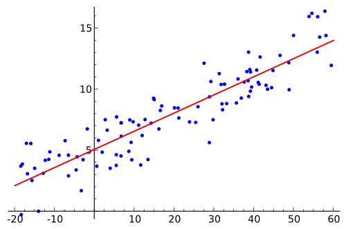
This is where the "magic" happens. The model tries to find the straight line that best fits the data points.

model = LinearRegression()

model.fit(X_train, y_train)

The .fit() method internally calculates the equation of the line, where the coefficient represents the salary increase for each additional year of experience.

6. Evaluation

Now we ask the model to predict the salaries for the data we saved in step 4 and compare its predictions with reality.

predictions = model.predict(X_test)

print(f"R²: {r2_score(y_test, predictions):.2f}")
print(f"MAE: {mean_absolute_error(y_test, predictions):.2f}")
print(f"RMSE: {np.sqrt(mean_squared_error(y_test, predictions)):.2f}")

Metric	What does it mean?
R²	How well the model explains the variance. 1.0 is perfect, 0.0 is like guessing randomly.
MAE	The average error in money. If it’s 500, the model is off by $500 on average.
RMSE	Similar to MAE, but penalizes large errors much more (the “outliers”).

If you want to learn more about metrics, read this: https://byandrev.dev/en/blog/performance-metrics-in-machine-learning .

7. Visualization

Finally, we plot the results.

plt.figure(figsize=(8,6))
sns.scatterplot(x=y_test, y=predictions, color='green')
plt.plot([y_test.min(), y_test.max()], [y_test.min(), y_test.max()], 'r--')

plt.xlabel("Real Salary")
plt.ylabel("Predicted Salary")
plt.title("Predicted vs Real - Linear Regression")
plt.grid(True)

plt.show()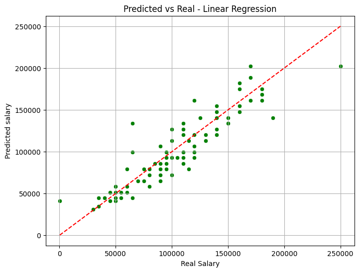

Linear Regression to Predict Salaries

Graph of a Linear Regression model.

The red line represents "perfection" (where the prediction equals reality). The closer the green points are to the red line, the better your model is.

Blog