Ads
A step-by-step exercise on how to classify customer reviews of products using NLP with the Naive Bayes classifier to determine if they are positive or negative.
I have been diving into Machine Learning, and in this exercise, I will use the Naive Bayes classifier to categorize user reviews as either positive or negative. Naive Bayes is an excellent starting point for this type of task, though it is worth noting that technologies like Transformers are often a better choice for modern applications.
Naive Bayes
Naive Bayes is a supervised classification algorithm used to predict which category a data point belongs to based on probabilities. The name comes from Bayes' Theorem, while "Naive" refers to the simplistic assumption underlying the logic.
Its main advantages are speed and efficiency. On the downside, its "naivety" assumes that words have no relationship with each other and does not account for word order. Despite this, the algorithm remains highly effective for cases such as:
- Spam filters.
- Sentiment analysis.
- Recommendation systems.
Required Libraries
You will need to install the following libraries. I recommend performing this exercise in Google Colab to simplify environment setup. Set the Runtime to T4 to handle the size of the CSV file.
- sklearn: Essential for text vectorization, model training, and calculating metrics.
- nltk: Used primarily for managing and filtering stopwords.
- spaCy: Our primary tool for tokenization.
- joblib: For saving and loading Machine Learning models.
Data Preparation
Loading the Dataset
You can download the dataset here: reviews.csv. The dataset contains 210,000 reviews with the following columns: stars, review_body, language, and product_category. All reviews are in Spanish.
import pandas as pd

df = pd.read_csv('reviews.csv')
Before cleaning the data, it is important to understand how our labels are distributed. We will visualize the frequency of scores to verify if we have a balanced dataset.
import matplotlib.pyplot as plt
import seaborn as sns

plt.figure(figsize=(8, 4))
sns.countplot(x='stars', data=df)
plt.title('Distribution of Scores')
plt.show()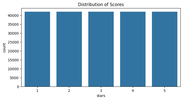
A significant imbalance (for example, having many 5-star reviews and almost no 1-star reviews) could bias our model's predictions. Our current dataset is well-balanced.
Removing Null Rows
It is necessary to clean the dataset by removing rows that do not contain complete information, as these can cause errors.
# Check the number of null values per column
df.isnull().sum()

# Remove rows containing null values
df.dropna(inplace=True)
Text Cleaning and Normalization
The next step is to standardize the content. We will create a cleaning function using regular expressions to remove noise from the data.
import re
import string

def preprocess_text(text):
    """
    Performs text cleaning: conversion to lowercase,
    noise removal (URLs, HTML, tags), and character normalization.
    """

    # Convert to lowercase
    text = str(text).lower()

    # Remove content within brackets (e.g., tags or references)
    text = re.sub(r'\[.*?\]', '', text)

    # Remove URLs and web addresses
    text = re.sub(r'https?://\S+|www\.\S+', '', text)

    # Remove HTML tags
    text = re.sub(r'<.*?>+', '', text)

    # Replace line breaks with spaces
    text = re.sub(r'\n', ' ', text)

    # Remove words containing digits
    text = re.sub(r'\w*\d\w*', '', text)

    # Remove extra whitespace
    text = text.strip()

    return text

df["clean_review"] = df["review_body"].apply(preprocess_text)
Removing Stopwords
This technique removes common words like "the," "is," or "of," which do not carry significant semantic meaning for classifying text.
By removing them, we increase processing speed and focus the model on important terms. However, this should be applied carefully; in certain contexts (like sentiment analysis), removing a negation can completely change the meaning of a sentence.
import nltk
from nltk.corpus import stopwords

# Download the Spanish stopwords corpus
nltk.download('stopwords')
stopword_es = set(stopwords.words('spanish'))- A corpus is a large, structured set of texts. In this case, we are downloading a predefined linguistic database from
nltk.
Tokenization and Lemmatization
For an algorithm to understand text, we must break it down and normalize it:
- Tokenization: The process of dividing text into smaller units called tokens. This is essential for word counting or vectorization.
- Lemmatization: Uses a dictionary to reduce each word to its linguistic root or "lemma." It is more precise than stemming and preserves meaning, though it is slower and requires more computational resources. Example: The verb forms "running," "runs," and "ran" are normalized to "run."
Why reduce the vocabulary? We aim to eliminate noise and improve efficiency. Every word becomes a column in our feature matrix. Through stopwords and lemmatization, we group terms to achieve better performance.
We need to download the specific language model for Spanish (es_core_news_sm):
!python -m spacy download es_core_news_smimport spacy
nlp_es = spacy.load('es_core_news_sm')
def clean(text):
"""
Applies tokenization, stopword removal, and lemmatization
using the spaCy model.
"""
doc = nlp_es(text)
# Filter by stopwords and extract the lemma for each token
lemmatized = [token.lemma_ for token in doc if token.text.lower() not in stopword_es]
return " ".join(lemmatized).strip()
# Apply the transformation to the DataFrame
df["clean_review"] = df["clean_review"].apply(clean)Vectorization with TF-IDF
At this stage, we transform text into numerical representations called vectors. While several methods exist, we will use TF-IDF (Term Frequency - Inverse Document Frequency).
TF-IDF measures not only how frequent a term is in a document but also how relevant it is compared to the entire dataset (corpus). This method is based on the Bag of Words model, which analyzes the importance of terms without considering their order or context.
from sklearn.feature_extraction.text import TfidfVectorizer

corpus = df["clean_review"].tolist()

tfidf = TfidfVectorizer()
tfidf_matrix = tfidf.fit_transform(corpus)

print(f"Matrix dimensions: {tfidf_matrix.shape}")
Naive Bayes Classifier
Now we will train and evaluate a Naive Bayes classifier to determine the sentiment (positive or negative) of the reviews.
First, we must construct our target variable: if a review has more than 3 stars, it will be labeled 1 (positive); if it has 3 or fewer, it will be 0 (negative).
df["sentiment"] = df["stars"].apply(lambda x: 1 if x > 3 else 0)Splitting the Dataset
To ensure our model can generalize to new data, we will split our dataset into two groups:
- Training set: The data the model uses to learn the relationships between words and sentiment.
- Test set: Data the model has never seen, used to validate its final accuracy.
from sklearn.model_selection import train_test_split

X = tfidf_matrix
y = df["sentiment"]

X_train, X_test, y_train, y_test = train_test_split(
    X,
    y,
    test_size=0.2,
    random_state=42
)- We reserve 20% of the dataset for the final test.
random_state=42ensures that if the code is run again, the split remains the same, making results reproducible.
Training
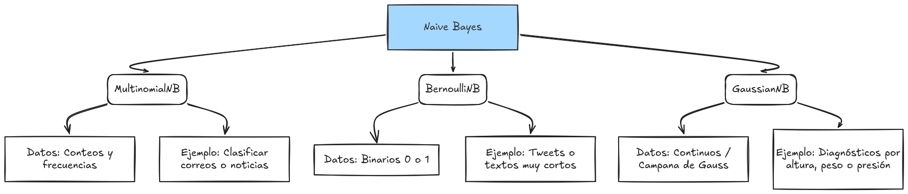
We will use MultinomialNB, a variant of the Naive Bayes algorithm specifically designed for discrete data like word counts or frequencies. It treats each word as an event occurring a certain number of times.
from sklearn.naive_bayes import MultinomialNB

nb_classifier = MultinomialNB()
nb_classifier.fit(X_train, y_train)
There are other options such as the following:
Model Evaluation
Once trained, we must measure how well our model performs. We will use several metrics:
- Accuracy: The percentage of total correct predictions.
- Precision: Indicates the quality of positive predictions. How reliable is the model when it says "positive"?
- Recall: Measures the model's ability to identify all actual positive cases.
from sklearn.metrics import accuracy_score, classification_report

y_pred = nb_classifier.predict(X_test)

print("Accuracy:", accuracy_score(y_test, y_pred))
print("Classification Report:\n", classification_report(y_test, y_pred))
If you want to learn more about metrics, check out this resource: https://byandrev.dev/en/blog/performance-metrics-in-machine-learning
Saving the Model
We will now save the model for future use using the joblib library.
import joblib

model_path = "/content/nb_classifier_model.pkl"
joblib.dump(nb_classifier, model_path)

print(f"Model exported successfully to: {model_path}")
Importing the Model
loaded_model = joblib.load(model_path)Testing with Real Data
For the model to understand a new sentence, it must undergo the same vectorization process (TF-IDF) used during training.
new_review = "Es un producto excelente, superó mis expectativas" # "It is an excellent product, it exceeded my expectations"

clean_review = clean(preprocess_text(new_review))
new_vector = tfidf.transform([clean_review])
prediction = loaded_model.predict(new_vector)

print(f"Review: '{new_review}'")
print(f"Sentiment Prediction: {prediction[0]}")Share this article on